Advanced Numerical Methods (ANM) in Python
ANM Usage Guide
Instructions of anm
- Download and move
anm.pyto package path or workspace - create a new Python file
*.pyor Ipython Notebook*.ipynbin workspace - start programing by importing
anmand essential packages, as shown below:import anm import numpy as np import matplotlib.pyplot as plt - Check the docstring for basic instructions
- Open docstring by placing your cursor on
anmor anm modules such asanm.linregrand pressShift+Tab - Get list of modules by placing your cursor to the end of
anm.and pressTab
![]()
ANM Guide
# Import the essential python packages
import anm
import numpy as np
import matplotlib.pyplot as plt
bisect
f_x = lambda x: 1*x**3 + 4*x**2 - 1
root, fx, ea, iter = anm.bisect(func = f_x, xl = 0, xu = 1, es = 1e-4, maxit = 50)
print('xr: {}\nf(xr): {}\nea: {}\niter: {}'.format(root, fx, ea, iter))
xr: 0.47283387184143066
f(xr): -1.654603528633558e-07
ea: 5.0423329059115807e-05
iter: 22
bisect2
f_x = lambda x: 1*x**3 + 4*x**2 - 1
xr, f_xr = anm.bisect2(func = f_x)
print('\nxr: {}\nf(xr): {}'.format(xr, f_xr))
enter lower bound xl = 0
enter upper bound xu = 1
allowable tolerance es = 1e-4
maximum number of iteration maxit = 50

Bisection method has converged

step	xl		xu		xr		f(xr)
1	0.00000000	1.00000000	0.50000000	0.12500000
2	0.00000000	0.50000000	0.25000000	-0.73437500
3	0.25000000	0.50000000	0.37500000	-0.38476562
4	0.37500000	0.50000000	0.43750000	-0.15063477
5	0.43750000	0.50000000	0.46875000	-0.01809692
6	0.46875000	0.50000000	0.48437500	0.05212021
7	0.46875000	0.48437500	0.47656250	0.01668024
8	0.46875000	0.47656250	0.47265625	-0.00079101
9	0.47265625	0.47656250	0.47460938	0.00792392
10	0.47265625	0.47460938	0.47363281	0.00356129
11	0.47265625	0.47363281	0.47314453	0.00138384
12	0.47265625	0.47314453	0.47290039	0.00029609
13	0.47265625	0.47290039	0.47277832	-0.00024754
14	0.47277832	0.47290039	0.47283936	0.00002426

xr: 0.47283935546875
f(xr): 2.4255414928120445e-05
false_position
f_x = lambda x: 1*x**3 + 4*x**2 - 1
xr, f_xr = anm.false_position(func = f_x)
print('\nxr: {}\nf(xr): {}'.format(xr, f_xr))
enter lower bound xl = 0
enter upper bound xu = 1
allowable tolerance es = 1e-4
maximum number of iteration maxit = 50

False position method has converged

step	xl		xu		xr		f(xr)
1	0.00000000	1.00000000	0.20000000	-0.83200000
2	0.20000000	1.00000000	0.33774834	-0.50517594
3	0.33774834	1.00000000	0.41200817	-0.25105836
4	0.41200817	1.00000000	0.44673371	-0.11256088
5	0.44673371	1.00000000	0.46187662	-0.04814781
6	0.46187662	1.00000000	0.46827694	-0.02018150
7	0.46827694	1.00000000	0.47094622	-0.00838731
8	0.47094622	1.00000000	0.47205323	-0.00347335
9	0.47205323	1.00000000	0.47251127	-0.00143627
10	0.47251127	1.00000000	0.47270061	-0.00059355
11	0.47270061	1.00000000	0.47277884	-0.00024523

xr: 0.4727788398539938
f(xr): -0.00024522776512281297
multiple1
f_x = lambda x: 1*x**3 + 4*x**2 - 1
df_x = lambda x: x*(3*x + 8)
xr, f_xr = anm.multiple1(f_x, df_x)
print('\nxr: {}\nf(xr): {}'.format(xr, f_xr))
Enter the multiplicity of the root = 1
Enter the initial guess for x = 10
Enter the allowable tolerance = 1e-4
Enter the maximum number of iterations = 50

Newton's method has converged.

Step	x		f		df/dx
1	10.00000000	1399.00000000	380.00000000
2	6.31842105	410.93659282	170.31470222
3	3.90561354	119.59078328	77.00635973
4	2.35261475	34.16042787	35.42530657
5	1.38832027	9.38562715	16.88886160
6	0.83259144	2.34999353	8.74035709
7	0.56372445	0.45028435	5.46315138
8	0.48130236	0.03810249	4.54537479
9	0.47291967	0.00038195	4.45431637
10	0.47283392	0.00000004	4.45338709

xr: 0.4728339179418582
f(xr): 3.9842684262936245e-08
multiple2
f_x = lambda x: 1*x**3 + 4*x**2 - 1
df_x = lambda x: x*(3*x + 8)
ddf_x = lambda x: 6*x + 8
xr, f_xr = anm.multiple2(f_x, df_x, ddf_x)
print('\nxr: {}\nf(xr): {}'.format(xr, f_xr))
Enter initial guess: xguess = 1
Allowable tolerance es = 1e-4
Maximum number of iterations: maxit = 50

Newton method has converged

Step	x		f		df/dx		d2f/dx2
1	1.00000000	4.00000000	11.00000000	14.00000000
2	0.32307692	-0.54876286	2.89775148	9.93846154
3	0.43788443	-0.14906772	4.07830378	10.62730659
4	0.47125720	-0.00700821	4.43630769	10.82754322
5	0.47283088	-0.00001351	4.45335412	10.83698526
6	0.47283391	-0.00000000	4.45338699	10.83700345

xr: 0.47283390898406397
f(xr): -4.9840465088379915e-11
newtraph
# Newton-Raphson method
f_x = lambda x: 1*x**3 + 4*x**2 - 1
df_x = lambda x: x*(3*x + 8)
root, ea, iter = anm.newtraph(func = f_x, dfunc = df_x, xr = 0.1, es = 1e-4, maxit = 50)
print('root: {}\nea: {}\niter: {}'.format(root, ea, iter))
root: 0.4728339089952555
ea: 1.425450195876832e-07
iter: 7
Cubic_LS
# Least Square Cubic Equation
a = np.array(range(10)).astype(np.float64)
b = 1+5*a**3
z, Syx, r = anm.Cubic_LS(a,b)
print(f'y = {z[0]:.4f} + {z[1]:.4f} *x + {z[2]:.4f} *x**2 + {z[3]:.4f} *x**3\n\nStandard Error: {Syx}\n\ncorr: {r}')
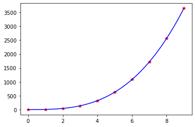
y = 1.0000 + -0.0000 *x + 0.0000 *x**2 + 5.0000 *x**3

Standard Error: 2.050454164737037e-10

corr: 1.0
Gauss_Newton
# Nonlinear Regression of f(x)=exp(-a0*x)cos(a1*x) using Gauss-Newton method
a = np.array(range(-10,10+1)).astype(np.float64)
b = np.exp(-2*a)*np.cos(5*a) # f(x)=exp(-a0*x)cos(a1*x)
a0, a1 = anm.Gauss_Newton(a, b)
print('f(x)=exp({:.1f}*x)*cos({:.1f}*x)'.format(a0, a1))
Enter the initial guess of a0 = 1.5
Enter the initial guess of a1 = 4.5
Enter the tolerance to1 = 1e-4
Enter the maximum iteration number itmax = 10

iter	a0		a1		da0		da1
0	1.87188241	-12.01705764	0.37188241	-16.51705764
1	2.17941947	-11.93159922	0.30753706	0.08545841
2	2.09424379	-11.95101275	-0.08517568	-0.01941353
3	2.03479081	-11.97112615	-0.05945297	-0.02011340
4	2.01178429	-11.98550069	-0.02300652	-0.01437454
5	2.00992858	-11.98882560	-0.00185572	-0.00332491
6	2.00997074	-11.98889115	0.00004216	-0.00006555

Gauss-Newton method has converged
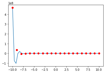
f(x)=exp(2.0*x)*cos(-12.0*x)
Lagrange_coef
# Lagrange coefficient
a = np.array(range(-8,8+1))
b = 1+5*a**3
c = anm.Lagrange_coef(a,b)
print(f'coef: {c}')
coef: [-1.27682557e-06  8.55157130e-07  6.21158512e-07 -4.82755097e-07
  2.29684201e-07  2.70680438e-07  2.31834945e-08  2.18708883e-09
  6.15118733e-10 -3.28063324e-09 -2.43723917e-08 -2.74720444e-07
 -2.31124227e-07  4.84302389e-07 -6.22309871e-07 -8.56154979e-07
  1.27782348e-06]
Lagrange_Eval
# Lagrange Evaluation
x = np.array([0, 1, 4, 3])
y = lambda x: np.exp(x)
c = anm.Lagrange_coef(x,y(x))
t = [2, 2.4, 2.6]
p = anm.Lagrange_Eval(t,x,c)
for i in range(len(t)):
    print('\nt = ',t[i])
    print('Lagr f(t): ',p[i])
    print('True f(t): ',y(t[i]))
t =  2
Lagr f(t):  5.936187495573769
True f(t):  7.38905609893065

t =  2.4
Lagr f(t):  9.75597209973619
True f(t):  11.023176380641601

t =  2.6
Lagr f(t):  12.510387425884225
True f(t):  13.463738035001692
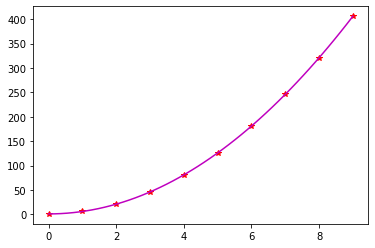
Linear_LS
# Least Square Linear Regression
x = np.array(range(10))
y = 1+5*x**2
[a0, a1], Syx, r = anm.Linear_LS(x,y)
print('y = {} + {} * x\nSyx: {}\nr2: {}'.format(float(a0), float(a1), Syx, r))
x		y		(a0+a1*x)	(y-a0-a1*x)
0.00000000	1.00000000	-59.00000000	60.00000000
1.00000000	6.00000000	-14.00000000	20.00000000
2.00000000	21.00000000	31.00000000	-10.00000000
3.00000000	46.00000000	76.00000000	-30.00000000
4.00000000	81.00000000	121.00000000	-40.00000000
5.00000000	126.00000000	166.00000000	-40.00000000
6.00000000	181.00000000	211.00000000	-30.00000000
7.00000000	246.00000000	256.00000000	-10.00000000
8.00000000	321.00000000	301.00000000	20.00000000
9.00000000	406.00000000	346.00000000	60.00000000
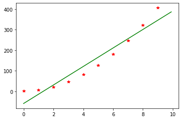
y = -59.0 + 45.0 * x
Syx: 40.620192023179804
r2: 0.9626907371412557
linregr
# Linear Regression
x = np.array(range(10))
y = 1+5*x**2
[a0, a1], r2 = anm.linregr(x,y)
print('y = {} + {} * x\nr2: {}'.format(float(a1), float(a0), r2))
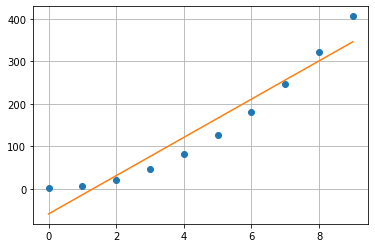
y = -59.0 + 45.0 * x
r2: 0.9267734553775746
Multiple_Linear
# Multi-linear Regression
x1 = np.arange(-10,10,0.8)
x2 = np.arange(-10,10,0.8)**3+2
y = 1+5*x1**2+x2
a0, a1, a2, Syx, r = anm.Multiple_Linear(x1, x2, y)
print(f'y = {a0:.4f} + {a1:.4f}*x1 + {a2:.4f}*x2\nSyx: {Syx}\nr2: {r}')
x1		x2		y		(a0+a1*x1+a2*x2)	(y-a0-a1*x1-a2*x2)
-10.00000000	-998.00000000	-497.00000000	-705.92903226		208.92903226
-9.20000000	-776.68800000	-352.48800000	-526.59552688		174.10752688
-8.40000000	-590.70400000	-236.90400000	-374.67604301		137.77204301
-7.60000000	-436.97600000	-147.17600000	-247.78675269		100.61075269
-6.80000000	-312.43200000	-80.23200000	-143.54382796		63.31182796
-6.00000000	-214.00000000	-33.00000000	-59.56344086		26.56344086
-5.20000000	-138.60800000	-2.40800000	6.53823656		-8.94623656
-4.40000000	-83.18400000	14.61600000	57.14503226		-42.52903226
-3.60000000	-44.65600000	21.14400000	94.64077419		-73.49677419
-2.80000000	-19.95200000	20.24800000	121.40929032		-101.16129032
-2.00000000	-6.00000000	15.00000000	139.83440860		-124.83440860
-1.20000000	0.27200000	8.47200000	152.29995699		-143.82795699
-0.40000000	1.93600000	3.73600000	161.18976344		-157.45376344
0.40000000	2.06400000	3.86400000	168.88765591		-165.02365591
1.20000000	3.72800000	11.92800000	177.77746237		-165.84946237
2.00000000	10.00000000	31.00000000	190.24301075		-159.24301075
2.80000000	23.95200000	64.15200000	208.66812903		-144.51612903
3.60000000	48.65600000	114.45600000	235.43664516		-120.98064516
4.40000000	87.18400000	184.98400000	272.93238710		-87.94838710
5.20000000	142.60800000	278.80800000	323.53918280		-44.73118280
6.00000000	218.00000000	399.00000000	389.64086022		9.35913978
6.80000000	316.43200000	548.63200000	473.62124731		75.01075269
7.60000000	440.97600000	730.77600000	577.86417204		152.91182796
8.40000000	594.70400000	948.50400000	704.75346237		243.75053763
9.20000000	780.68800000	1204.88800000	856.67294624		348.21505376
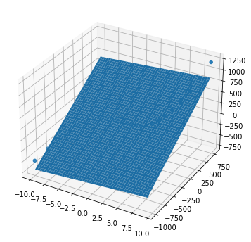
y = 163.4867 + 9.4982*x1 + 0.7760*x2
Syx: 153.96086641447857
r2: 0.9227306867620393
Newtint2
# Newton Interpolating Polynomial
x = np.linspace(10, 50, 50)
y = lambda x: x**2 + 10
xx = [30, 43.45]
b, yint = anm.Newtint2(x, y(x), xx)
for i in range(len(xx)):
    print('\nxx = ',xx[i])
    print('inter yy = ',yint[i])
    print('true  yy = ',y(xx[i]))
xx =  30
inter yy =  909.9999999999994
true  yy =  910

xx =  43.45
inter yy =  1897.9024999999954
true  yy =  1897.9025000000001
quadratic
# Quadratic
x = np.array([-1, 0, 2, 5, 6])
f = x**3 - 5*x**2 + 3*x + 4
print('f = ',f)
A, b = anm.quadratic(x, f)
print('\nA:\n{}\n\nb: {}'.format(A, b))
f =  [-5  4 -2 19 58]

A:
[[ 1  0  0  0  0  0  0  0  0  0  0  0]
 [ 0  1  1  0  0  0  0  0  0  0  0  0]
 [ 0  0  0  1  0  0  0  0  0  0  0  0]
 [ 0  0  0  0  2  4  0  0  0  0  0  0]
 [ 0  0  0  0  0  0  1  0  0  0  0  0]
 [ 0  0  0  0  0  0  0  3  9  0  0  0]
 [ 0  0  0  0  0  0  0  0  0  1  0  0]
 [ 0  0  0  0  0  0  0  0  0  0  1  1]
 [ 0  1  2  0 -1  0  0  0  0  0  0  0]
 [ 0  0  0  0  1  4  0 -1  0  0  0  0]
 [ 0  0  0  0  0  0  0  1  6  0 -1  0]
 [ 0  0  1  0  0  0  0  0  0  0  0  0]]

b: [-5  9  4 -6 -2 21 19 39  0  0  0  0]
Quadratic_LS
# Quadratic Least Square
x = np.array(range(10)).astype(np.float64)
y = 1+5*x**2
z, Syx, r = anm.Quadratic_LS(x,y)
print('y = {:.4f} + {:.4f} *x + {:.4f} *x**2\nSyx: {}\nr:{}'.format(float(z[0]), float(z[1]), float(z[2]), Syx, r))
x		y		(a0+a1*x+a2*x**2)	(y-a0-a1*x-a2*x**2)
0.00000000	1.00000000	1.00000000		-0.00000000
1.00000000	6.00000000	6.00000000		-0.00000000
2.00000000	21.00000000	21.00000000		-0.00000000
3.00000000	46.00000000	46.00000000		-0.00000000
4.00000000	81.00000000	81.00000000		-0.00000000
5.00000000	126.00000000	126.00000000		-0.00000000
6.00000000	181.00000000	181.00000000		0.00000000
7.00000000	246.00000000	246.00000000		0.00000000
8.00000000	321.00000000	321.00000000		0.00000000
9.00000000	406.00000000	406.00000000		0.00000000
y = 1.0000 + -0.0000 *x + 5.0000 *x**2
Syx: 2.6933640544107207e-14
r:1.0
Cholesky
# Cholesky Decomposition
A = np.array([[6,  15, 55],
              [15, 55, 225],
              [55, 225,979]]) # must be symmetric matrix
L, U = anm.Cholesky(A)
print('A :\n',A,'\n\nL :\n',L,'\n\nU :\n',U)
A :
 [[  6  15  55]
 [ 15  55 225]
 [ 55 225 979]]

L :
 [[ 2.44948974  0.          0.        ]
 [ 6.12372436  4.18330013  0.        ]
 [22.45365598 20.91650066  6.11010093]]

U :
 [[ 2.44948974  6.12372436 22.45365598]
 [ 0.          4.18330013 20.91650066]
 [ 0.          0.          6.11010093]]
# test
L @ U # dot product
array([[  6.,  15.,  55.],
       [ 15.,  55., 225.],
       [ 55., 225., 979.]])
GaussNaive
# Naive Gauss elimination
# solving equations:
# x1 + 2*x3 + 3*x4 = 1
# -x1 + 2*x2 + 2*x3 - 3*x4 = -1
# x2 + x3 + 4*x4 = 2
# 6*x1 + 2*x2 + 2*x3 + 4*x4 = 1
A = np.array([[1, 0, 2, 3],
              [-1, 2, 2, -3],
              [0, 1, 1, 4],
              [6, 2, 2, 4]])
b = np.array([1, -1, 2, 1])
x = anm.GaussNaive(A, b)
x
array([-0.18571429, 0.22857143, -0.11428571, 0.47142857])
GaussPivot
# Gauss elimination with pivoting
# solving equations:
# x1 + 2*x3 + 3*x4 = 1
# -x1 + 2*x2 + 2*x3 - 3*x4 = -1
# x2 + x3 + 4*x4 = 2
# 6*x1 + 2*x2 + 2*x3 + 4*x4 = 1
A = np.array([[1, 0, 2, 3],
              [-1, 2, 2, -3],
              [0, 1, 1, 4],
              [6, 2, 2, 4]])
b = np.array([1, -1, 2, 1])
x = anm.GaussPivot(A, b)
x
array([-0.18571429, 0.22857143, -0.11428571, 0.47142857])
LU_factor
# Direct LU factorization
A = np.array([[-19, 20, -6],
              [-12, 13, -3],
              [30, -30, 12]])
L, U = anm.LU_factor(A)
print('L :\n',L,'\n\nU :\n',U)
L :
 [[ 1.          0.          0.        ]
 [ 0.63157895  1.          0.        ]
 [-1.57894737  4.28571429  1.        ]]

U :
 [[-19.          20.          -6.        ]
 [  0.           0.36842105   0.78947368]
 [  0.           0.          -0.85714286]]
LU_pivot
# Pivot LU factorization
A = np.array([[-19, 20, -6],
              [-12, 13, -3],
              [30, -30, 12]])
L, U, P = anm.LU_pivot(A)
print('A :\n',A,'\n\nL :\n',L,'\n\nU :\n',U,'\n\nP :\n',P,'\n\nL*U :\n',L@U,'\n\nP*A :\n',P@A)
A :
 [[-19  20  -6]
 [-12  13  -3]
 [ 30 -30  12]]

L :
 [[ 1.          0.          0.        ]
 [-0.4         1.          0.        ]
 [-0.63333333  1.          1.        ]]

U :
 [[ 30 -30  12]
 [  0   1   1]
 [  0   0   0]]

P :
 [[0. 0. 1.]
 [0. 1. 0.]
 [1. 0. 0.]]

L*U :
 [[ 30.  -30.   12. ]
 [-12.   13.   -3.8]
 [-19.   20.   -6.6]]

P*A :
 [[ 30. -30.  12.]
 [-12.  13.  -3.]
 [-19.  20.  -6.]]
LU_Solve
# Function to solve the equation LUx=b
# solving equations:
# x1 + 2*x3 + 3*x4 = 1
# -x1 + 2*x2 + 2*x3 - 3*x4 = -1
# x2 + x3 + 4*x4 = 2
# 6*x1 + 2*x2 + 2*x3 + 4*x4 = 1
A = np.array([[1, 0, 2, 3],
              [-1, 2, 2, -3],
              [0, 1, 1, 4],
              [6, 2, 2, 4]])
b = np.array([1, -1, 2, 1])
L, U = anm.LU_factor(A)
x = anm.LU_Solve(L, U, b)
x
array([-0.18571429, 0.22857143, -0.11428571, 0.47142857])
Tridiag
# Tridiagonal matrix
e = np.array([0, -2, 4, -0.5, 1.5, -3])
f = np.array([1, 6, 9, 3.25, 1.75, 13])
g = np.array([-2, 4, -0.5, 1.5, -3, 0])
r = np.array([-3, 22, 35.5, -7.75, 4, -33])
anm.Tridiag(e, f, g, r)
[1.0, 2.0, 3.0, -1.0, -2.0, -3.0]
Truss
# Truss
A, b, f = anm.Truss(alpha = np.pi/6, beta = np.pi/3, gamma = np.pi/4, delta = np.pi/3)
print('A :\n',A,'\n\nb :\n',b,'\n\nf :\n',f)
A :
 [[ 1.          0.          0.          0.          0.5         0.
   0.          0.          0.          0.        ]
 [ 0.          1.          0.          1.          0.8660254   0.
   0.          0.          0.          0.        ]
 [ 0.          0.          0.          0.          0.          0.
   0.8660254   0.70710678  0.          0.        ]
 [ 0.          0.          0.         -1.          0.          1.
  -0.5         0.70710678  0.          0.        ]
 [ 0.          0.          1.          0.          0.          0.
   0.          0.          0.70710678  0.        ]
 [ 0.          0.          0.          0.          0.         -1.
   0.          0.         -0.5         0.        ]
 [ 0.          0.          0.          0.         -0.5         0.
  -0.8660254   0.          0.          0.        ]
 [ 0.          0.          0.          0.         -0.8660254   0.
   0.5         0.          0.          1.        ]
 [ 0.          0.          0.          0.          0.          0.
   0.         -0.70710678 -0.8660254   0.        ]
 [ 0.          0.          0.          0.          0.          0.
   0.         -0.70710678  0.5        -1.        ]]

b :
 [[  0.]
 [  0.]
 [100.]
 [  0.]
 [  0.]
 [  0.]
 [  0.]
 [  0.]
 [  0.]
 [  0.]]

f :
 [[ 4.05827420e+01]
 [ 2.84217094e-14]
 [ 4.85139880e+01]
 [ 7.02913710e+01]
 [-8.11654839e+01]
 [ 3.43045699e+01]
 [ 4.68609140e+01]
 [ 8.40286922e+01]
 [-6.86091399e+01]
 [-9.37218280e+01]]
fixed_pt_sys
# Fixed-point method
def fp_examp_1(x):
    return np.array([-0.02*x[0]**2 - 0.02*x[1]**2 - 0.02*x[2]**2 + 4,
                     -0.05*x[0]**2 - 0.05*x[2]**2 + 2.5,
                     -0.025*x[0]**2 + 0.025*x[1]**2 - 1.875])
x = anm.fixed_pt_sys(fp_examp_1, x0 = [0, 0, 0], es = 1e-4, maxit = 50)
print('x :',x)
iter	 x[0]		x[1]		x[2] 		diff
1	 4.00000000	2.50000000	-1.87500000 	5.07598513
2	 3.48468750	1.52421875	-2.11875000 	1.13009295
3	 3.62089217	1.66839257	-2.12049510 	0.19834528
4	 3.59218213	1.61963202	-2.13318316 	0.05799004
5	 3.59845099	1.62728786	-2.13201411 	0.00996379
6	 3.59715201	1.62528332	-2.13251959 	0.00244152
7	 3.59742623	1.62564288	-2.13244892 	0.00045769
8	 3.59736943	1.62555930	-2.13246902 	0.00010303
9	 3.59738132	1.62557545	-2.13246559 	0.00002035

Fixed-point iteration has converged

x : [ 3.59738132  1.62557545 -2.13246559]
GaussSeidel
# Gauss Seidel method
A = np.array([[4, -1, -1], [6, 8, 0], [-5, 0, 12]], dtype=float)
b = np.array([-2, 45, 80])
x = anm.GaussSeidel(A, b, es=0.00001, maxit=50)
for i in range(len(x)):
    print(f'x{str(i+1)}: {float(x[i]):.8}')
iter	x[0]		x[1]		x[2]
1 	 2.61458333	3.66406250	7.75607639
2 	 2.35503472	3.85872396	7.64793113
3 	 2.37666377	3.84250217	7.65694324
4 	 2.37486135	3.84385399	7.65619223
5 	 2.37501155	3.84374133	7.65625481
6 	 2.37499904	3.84375072	7.65624960
7 	 2.37500008	3.84374994	7.65625003
8 	 2.37499999	3.84375001	7.65625000

Gauss Serdel method has converged

x1: 2.375
x2: 3.84375
x3: 7.65625
InvPower
# Inverse Power Method
A = np.array([[2, 8, 10], [8, 3, 4], [10, 4, 7]])
z, m, error = anm.InvPower(A, max_it = 100, tol = 1e-3)
print('\nz :\n',z,'\n\nm :',float(m),'\n\nerror :',error)
iter	m		z[0]		z[1]		z[2]
1 	12.78260870	0.30000000	1.00000000	-0.53333333
2 	0.71234406	0.12048504	1.00000000	-0.80134159
3 	0.66865130	0.11674049	1.00000000	-0.81523988
4 	0.66859469	0.11630856	1.00000000	-0.81545592

z :
 [[ 0.11630856]
 [ 1.        ]
 [-0.81545592]]

m : 0.6685946897500895

error : 0.0003163103147705191
LU_Solve_Gen
# Solve the equation using LUx=B
A = np.array([[-19, 20, -6],
              [-12, 13, -3],
              [30, -30, 12]])
L, U = anm.LU_factor(A)
B = np.eye(3)
x = anm.LU_Solve_Gen(L, U, B)
print('Inverse from LU_Solve_Gen :\n',x,'\n\nInverse of A :\n',np.linalg.inv(A))
Inverse from LU_Solve_Gen :
 [[ 11.         -10.           3.        ]
 [  9.          -8.           2.5       ]
 [ -5.           5.          -1.16666667]]

Inverse of A :
 [[ 11.         -10.           3.        ]
 [  9.          -8.           2.5       ]
 [ -5.           5.          -1.16666667]]
Newton_sys
# Solve the nonlinear system F(x) = 0 using Newton's method
def example_1(x):
    return np.array([x[0]**2 + x[1]**2 - 1,
                     x[0]**2 - x[1]])
def examp_1_j(x):
    return np.array([[2*x[0], 2*x[1]],
                     [2*x[0], -1]])
x = anm.Newton_sys(example_1, examp_1_j, x0 = [0.5, 0.5], tol = 1e-6, maxit = 100)
print(f'x1 = {x[0]:f} \nx2 = {x[1]:f}')
iter	x[0]		x[1]		diff
1 	 0.87500000	0.62500000 	0.39528471
2 	 0.79067460	0.61805556 	0.08461086
3 	 0.78616432	0.61803399 	0.00451034
4 	 0.78615138	0.61803399 	0.00001294
5 	 0.78615138	0.61803399 	0.00000000

Newton method has converged

x1 = 0.786151
x2 = 0.618034
Power_eig
# Power Method for finding eigenvalues
A = np.array([[2, 8, 10],[8, 3, 4],[10, 4, 7]])
z, m, error = anm.Power_eig(A, max_it = 100, tol = 1e-3)
print(f'\nz :{z.T}\nm : {float(m):.8f}\nerror : {error:.8f}')
iter	m		z[0]		z[1]		z[2]
1	21.000000	0.95238095	0.71428571	1.00000000
2	19.380952	0.90909091	0.71007371	1.00000000
3	18.931204	0.92433485	0.70798183	1.00000000
4	19.075276	0.91807450	0.70869876	1.00000000
5	19.015540	0.92060173	0.70840440	1.00000000
6	19.039635	0.91957849	0.70852341	1.00000000
7	19.029879	0.91999243	0.70847526	1.00000000
8	19.033825	0.91982492	0.70849474	1.00000000
9	19.032228	0.91989270	0.70848686	1.00000000

z :[[0.9198927  0.70848686 1.        ]]
m : 19.03222820
error : 0.00083175
SOR
# Successive Over Relaxation (SOR)
A = np.array([[4, -1, -1],
              [6, 8, 0],
              [-5, 0, 12]], dtype=float)
b = np.array([-2, 45, 80])
x0 = np.array([0, 0, 0], dtype=float)
anm.SOR(A, b, x0, w = 1.2, tol = 1e-6, max_it = 100)
iter	x[0]		x[1]		x[2]
1	-0.60000000	7.29000000	7.70000000
2	4.01700000	1.67670000	8.46850000
3	1.64016000	4.93851600	7.12638000
4	2.69143680	3.34000368	7.92044240
5	2.23984646	4.06613745	7.53583475
6	2.43262237	3.74741238	7.70914423
7	2.35044251	3.88511926	7.63339241
8	2.38546500	3.82605765	7.66605402
9	2.37054050	3.85130202	7.65205945
10	2.37690034	3.84052929	7.65803828
11	2.37419020	3.84512296	7.65548745
12	2.37534508	3.84316484	7.65657505
13	2.37485295	3.84399938	7.65611146
14	2.37506266	3.84364373	7.65630904
15	2.37497330	3.84379529	7.65622484
16	2.37501138	3.84373070	7.65626072
17	2.37499515	3.84375822	7.65624543
18	2.37500207	3.84374650	7.65625195
19	2.37499912	3.84375149	7.65624917
20	2.37500038	3.84374936	7.65625035
21	2.37499984	3.84375027	7.65624985

SOR method converged


array([2.37500007, 3.84374988, 7.65625006])
Gauss_quad
# Gauss Quadrature
def example1(x):
    return x**2*np.sin(2*x)
anm.Gauss_quad(f = example1 , a = 0, b = np.pi, k = 2)
-8.687766227719367
anm.Gauss_quad(f = example1 , a = 0, b = np.pi, k = 5)
-4.9333450976919435
quadadapt
# Adaptive Quadrature Formulation
def example1(x):
    return x**2*np.sin(2*x)
anm.quadadapt(f = example1, a = 0, b = np.pi)
-4.934802202223205
romberg
# Romberg Integration
def example1(x):
    return x**2*np.sin(2*x)
q, ea, iter = anm.romberg(func = example1, a = 0, b = np.pi, es = 1e-6, maxit = 50)
print(f'q : {q}\nea : {ea}\niter : {iter}')
q : -4.93480220056642
ea : 3.7448974908415425e-10
iter : 6
Simp
# Composite Simpson's Rule
def example2(x):
    return x*np.exp(2*x)
anm.Simp(f = example2, a = 0, b = 4, n = 2)
8240.411432288045
anm.Simp(f = example2, a = 0, b = 4, n = 4)
5670.9754315360115
anm.Simp(f = example2, a = 0, b = 4, n = 8)
5256.753502612332
anm.Simp(f = example2, a = 0, b = 4, n = 16)
5219.6754602990595
trap
# Composite Trapezoidal Rule
def example2(x):
    return x*np.exp(2*x)
anm.trap(func = example2, a = 0, b = 4, n = 1)
23847.663896333826
anm.trap(func = example2, a = 0, b = 4, n = 2)
12142.22454829949
anm.trap(func = example2, a = 0, b = 4, n = 4)
7288.787710726881
anm.trap(func = example2, a = 0, b = 4, n = 8)
5764.762054640969
anm.trap(func = example2, a = 0, b = 4, n = 16)
5355.947108884538
trapuneq
# Trapezoidal Rule for Unequally spaced data
x = np.array([0, 1, 1.5, 2.0, 2.5, 3.0, 3.3, 3.6, 3.8, 3.9, 4.0])
y = lambda x: x*np.exp(2*x)
anm.trapuneq(x, y(x))
5365.065050065013
Euler_sys
# Euler's Method for a System of ODEs
def example5(t, y):
    f1 = -0.5*y[0]
    f2 = 4 - 0.1*y[0] - 0.3*y[1]
    return np.array([f1, f2]).T
t, y = anm.Euler_sys(f = example5, tspan = np.array([0, 1]), y0 = np.array([4, 6]), h = 0.5)
print(f'\nt : {t}\ny : {y}')
t	y0		y1
0.0	4.00000000	6.00000000
0.5	3.00000000	6.90000000
1.0	2.25000000	7.71500000

t : 1.0
y : [2.25  7.715]
t, y = anm.Euler_sys(f = example5, tspan = np.array([0, 1]), y0 = np.array([4, 6]), h = 0.2)
print(f'\nt : {t}\ny : {y}')
t	y0		y1
0.0	4.00000000	6.00000000
0.2	3.60000000	6.36000000
0.4	3.24000000	6.70640000
0.6	2.91600000	7.03921600
0.8	2.62440000	7.35854304
1.0	2.36196000	7.66454246

t : 1.0
y : [2.36196    7.66454246]
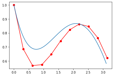
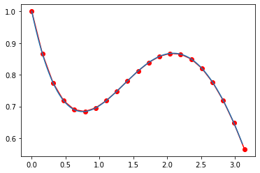
eulode
# Euler's method to integrate an ODE
dydt = lambda t,y: np.sin(t)-y
t, y = anm.eulode(dydt, tspan = np.array([0, np.pi]), y0 = 1, h = 0.1*np.pi)
step	t		y
1	0.00000000	1.00000000
2	0.31415927	0.68584073
3	0.62831853	0.56745807
4	0.94247780	0.57384404
5	1.25663706	0.64772580
6	1.57079633	0.74301996
7	1.88495559	0.82375262
8	2.19911486	0.86374632
9	2.51327412	0.84655259
10	2.82743339	0.76525844
11	3.14159265	0.62192596
tt = np.arange(0,np.pi,0.01*np.pi)
ye = 1.5*np.exp(-tt)+0.5*np.sin(tt)-0.5*np.cos(tt)
plt.plot(t, y, 'r-o', tt, ye)
plt.show()
example2_e
# Compute: 1.5 * np.exp(-t) + 0.5 * np.sin(t) - 0.5 * np.cos(t)
anm.example2_e(t = 1.25)
0.7465883237704438
# Alternative
def example2_e(t):
    return 1.5 * np.exp(-t) + 0.5 * np.sin(t) - 0.5 * np.cos(t)
example2_f
# Compute: np.sin(t) - y
anm.example2_f(t = 0, y = 1)
-1.0
# Alternative
def example2_f(t, y):
    return np.sin(t) - y
example3
# Compute: t * y**0.5
anm.example3(t = 1, y = 2)
1.4142135623730951
# Alternative
def example3(t, y):
    return t * y**0.5
example5
# Compute: [(-0.5 * y[0]), (4 - 0.1 * y[0] - 0.3 * y[1])]
anm.example5(y = [0.2, 0.3])
array([-0.1 , 3.89])
# Alternative
def example5(t, y):
    f1 = -0.5 * y[0]
    f2 = 4 - 0.1 * y[0] - 0.3 * y[1]
    return np.array([f1, f2], dtype=float)
Heun_iter
# Heun's iterative method (second order RK)
t, y = anm.Heun_iter(anm.example2_f, tspan = [0, np.pi], y0 = 1, h = 0.1*np.pi, itmax = 0) # without iteration
print(f'\nt : {t[-1]}\ny(t) : {y[-1]}')
t		y(t)
0.00000000	1.00000000
0.31415927	0.78372903
0.62831853	0.70180876
0.94247780	0.70636506
1.25663706	0.75585996
1.57079633	0.81523823
1.88495559	0.85647720
2.19911486	0.85921135
2.51327412	0.81116832
2.82743339	0.70822516
3.14159265	0.55397007

t : 3.141592653589793
y(t) : 0.5539700698900489
t, y = anm.Heun_iter(anm.example2_f, tspan = [0, np.pi], y0 = 1, h = 0.1*np.pi, itmax = 5) # with iteration
print(f'\nt : {t[-1]}\ny(t) : {y[-1]}')
t		y(t)
0.00000000	1.00000000
0.31415927	0.77043891
0.62831853	0.68300141
0.94247780	0.68718208
1.25663706	0.73954394
1.57079633	0.80361619
1.88495559	0.85029235
2.19911486	0.85836862
2.51327412	0.81493619
2.82743339	0.71541849
3.14159265	0.56312591

t : 3.141592653589793
y(t) : 0.563125910960438
Midpoint
# Midpoint method (second order RK)
t, y = anm.midpoint(anm.example2_f, tspan = [0, np.pi], y0 = 1, h = 0.05*np.pi)
print(f'\nt : {t[-1]}\ny(t) : {y[-1]}')
step	t		y(t)
1	0.00000000	1.00000000
2	0.15707963	0.86758170
3	0.31415927	0.77674522
4	0.47123890	0.72061651
5	0.62831853	0.69278558
6	0.78539816	0.68727353
7	0.94247780	0.69851646
8	1.09955743	0.72136291
9	1.25663706	0.75108125
10	1.41371669	0.78337410
11	1.57079633	0.81439677
12	1.72787596	0.84077724
13	1.88495559	0.85963533
14	2.04203522	0.86859892
15	2.19911486	0.86581568
16	2.35619449	0.84995869
17	2.51327412	0.82022492
18	2.67035376	0.77632578
19	2.82743339	0.71846924
20	2.98451302	0.64733328
21	3.14159265	0.56403095

t : 3.141592653589793
y(t) : 0.5640309524346758
tt = np.arange(0,np.pi,0.01*np.pi)
ye = 1.5*np.exp(-tt)+0.5*np.sin(tt)-0.5*np.cos(tt)
plt.plot(t, y, 'r-o', tt, ye)
plt.show()
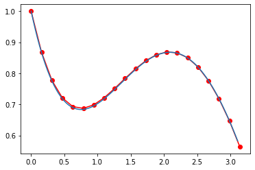
RK4
# Fouth-Order Runge-Kutta Method (RK4)
t, y = anm.RK4(anm.example2_f, tspan = [0, np.pi], y0 = 1, h = 0.05*np.pi)
print(f'\nt : {t[-1]}\ny(t) : {y[-1]}')
step	t		y(t)
1	0.00000000	1.00000000
2	0.15707963	0.86632848
3	0.31415927	0.77458664
4	0.47123890	0.71783758
5	0.62831853	0.68961947
6	0.78539816	0.68391042
7	0.94247780	0.69511065
8	1.09955743	0.71803843
9	1.25663706	0.74793644
10	1.41371669	0.78048517
11	1.57079633	0.81182074
12	1.72787596	0.83855431
13	1.88495559	0.85779080
14	2.04203522	0.86714487
15	2.19911486	0.86475244
16	2.35619449	0.84927613
17	2.51327412	0.81990370
18	2.67035376	0.77633854
19	2.82743339	0.71878178
20	2.98451302	0.64790575
21	3.14159265	0.56481903

t : 3.141592653589793
y(t) : 0.5648190301307761
tt = np.arange(0,np.pi,0.01*np.pi)
ye = 1.5*np.exp(-tt)+0.5*np.sin(tt)-0.5*np.cos(tt)
plt.plot(t, y, 'r-o', tt, ye)
plt.show()
RK4_sys
# 4th-order Runge-Kutta Method for ODEs
def example5(t, y):
    f1 = -0.5 * y[0]
    f2 = 4 - 0.1 * y[0] - 0.3 * y[1]
    return np.array([f1, f2], dtype=float)
t, y =anm.RK4_sys(example5, tspan = [0, 10], y0 = [4, 6], h = 0.5)
t	y[0]		y[1]
0.0	4.00000000	6.00000000
0.5	3.11523438	6.85767031
1.0	2.42617130	7.63210567
1.5	1.88952306	8.32688598
2.0	1.47157680	8.94686510
2.5	1.14607666	9.49760136
3.0	0.89257435	9.98495402
3.5	0.69514457	10.41480356
4.0	0.54138457	10.79286351
4.5	0.42163495	11.12455943
5.0	0.32837293	11.41495670
5.5	0.25573966	11.66872321
6.0	0.19917224	11.89011655
6.5	0.15511705	12.08298814
7.0	0.12080649	12.25079844
7.5	0.09408514	12.39663922
8.0	0.07327431	12.52325988
8.5	0.05706666	12.63309556
9.0	0.04444401	12.72829579
9.5	0.03461338	12.81075234
10.0	0.02695719	12.88212596
example1_f
# Compure: [y[1], -htc * (Ta - y[0])]
anm.example1_f([1, 0])
[0, -0.19]
# Alternative
def example1_f(y):
    htc = 0.01
    Ta = 20
    f1 = y[1]
    f2 = -htc * (Ta - y[0])
    return [f1, f2]
example3_f
# Compure: [y[1], -htc * (Ta**4 - y[0]**4)]
anm.example3_f([1, 0])
[0, -0.00799995]
# Alternative
def example3_f(y):
    htc = 5 * 10**(-8)
    Ta = 20
    f1 = y[1]
    f2 = -htc * (Ta**4 - y[0]**4)
    return [f1, f2]
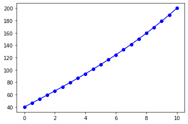
linear_FD
# Linear Finite-difference Method
x, y = anm.linear_FD()
left boundary aa = 0
right boundary bb = 10
number of subintervals n = 20
left boundary condition ya = 40
right boundary condition yb = 200
function p(x) = 0*x
function q(x) = 0.01*x**0
function r(x) = -0.01*20*x**0

x	y
0.0	40.00000000
0.5	46.37318260
1.0	52.81229815
1.5	59.33344445
2.0	65.95292436
2.5	72.68728658
3.0	79.55336701
3.5	86.56833087
4.0	93.74971555
4.5	101.11547452
5.0	108.68402218
5.5	116.47427989
6.0	124.50572330
6.5	132.79843102
7.0	141.37313482
7.5	150.25127145
8.0	159.45503627
8.5	169.00743867
9.0	178.93235967
9.5	189.25461157
10.0	200.00000000
shoot_secant
# Nonlinear shooting method based on secant method
def f(x, y, z):
    return np.array([z, -2*x*z/(1+x**2) - y/(1+x**2)])
anm.shooting_method_secant(x0 = 40, y0 = 4, y1 = 8, z0 = 200, f=f, tol=1e-6, max_iter=100)
120.01199999986355
# anm.shoot_secant() requires debugging